
In this note, we will give a generalization of Hsiung-Minkowski formulas for hypersurfaces in space forms. This will generalize the results in some of our previous posts. For example, as a special case of Theorem 6, we have the following result:
 is a space form,
  is a closed oriented hypersurface. Assume
 and
and
The definition of 


Corollary 2 (Corollary 13) Suppose is a closed hypersurface with
and
. Then
and
Here
and
is the region enclosed by
. The equality occurs if and only if
.


As another corollary, we have the following extension of Alexandrov’s theorem:
Corollary 3 (Corollary 11) Suppose . Assume
,
and there exists
such that
is constant where
is the distance from
The rest of this note is organized as follows. In Section 1 we will give the necessary definitions and preliminary results. In Section 2, we will prove the main results, and several corollaries will be given in Section 3.
1. Preliminaries
Let 


We define the 

If
We also define 


In the codimension one case, i.e. 
where 
Following [Grosjean] and [Reilly1], we define the (generalized) 

If

If

We also define 

This definition of
We collect some basic properties of
 .
.
 . i.e.
  (Here
(Here  If
If 
Proof: These equations are well-known, at least in the codimension one case (e.g. [Mar] Lemma 2.1). They can be found e.g. in [Grosjean] Lemma 2.1, 2.2 and [K1] Lemma 2.1. For (4), if 


2. Main results
In this section, we will first derive a simple integral formula and draw a few direct consequences. We will use the notations in Section 1. Throughout this section, we will also assume that 
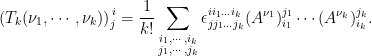
 be a symmetric
 is the
  -tensor defined by
  ,
,  (resp.
  ) is the tangential (resp. perpendicular) component of
  is the Lie derivative of
 Proof: Let 


The result follows by applying divergence theorem.
To proceed, let us recall that a vector field 
for some function 


We now state and prove our first main result.
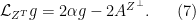
Theorem 6 Suppose is a conformal vector field along
- If
is even, then
- If
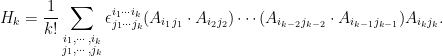
Here
and
are scalars,
-tensor, and


Proof: Recall that 

In general, it does not make sense to talk about 


Instead, we will now take a different approach to derive a formula similar to (3) for odd 


and
Similar to Lemma 4, we have
Lemma 7 For , we have (
denotes the trace on
 .
.
 are parallel in the normal bundle, then
  . i.e.

Proof: The proof is exactly the same as in the codimension one case of Lemma 4, see e.g. [Mar] Lemma 2.1, except that in (7), we need the fact that 
By applying Proposition 5 to 
Theorem 8 Suppose are (not necessarily distinct) normal fields to

Remark 1 If
3. Some examples and applications
By substituting different functions
Corollary 9 Suppose
- For all odd
, we have
Here we regard
- If
, we have
Here we regard
Proof: This follows from Theorem 6 by putting 


Corollary 10 Suppose . Assume that
, then we have
and
where
.


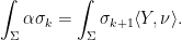
Proof: The first equation follows from Theorem 6 and the observation that 

We have the following extension of Alexandrov’s theorem.
 .
.
Proof: Assume 


where

By Proposition 12 below, 


Proposition 12 Suppose , then
where
Proof: By [Mar] Proposition 3.2, we have 

By a result of Ros ([Ros] Theorem 1), we have 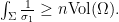
If one of the equality 

 and
and 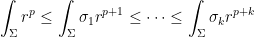


Proof: By [Mar] Proposition 3.2, if 


Remark 2 Corollary 13 generalizes [K1] Theorem 3.2 (1) and also [K2] Theorem 2.
To state our next result, we first set up the notations. We define 


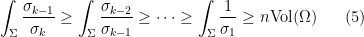
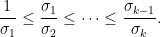
Let us recall that the classical Hsiung-Minkowski formulas [Hsiung]: if 


It is a nice observation that in general, if 


Therefore
In the following, we will consider the special case where the conformal vector field 


It is easily shown that the second fundamental form of 


In particular, for

By Theorem 6, Theorem 8, and in view of (9), we have the following result:
Theorem 14 Let be fixed and
be given by (8).
- If
- If
Here
- If there exists (not necessarily distinct) normal fields


In the following, we will apply Theorem 14 to 

Let us consider the case where 


By Theorem 14 and the above, we have
Corollary 15 With the notations above, let and

By substituting different functions
Corollary 16 With the same assumptions as in Corollary 15, suppose , then we have
and
where
.


Proof: The first equation follows by putting 


Corollary 17 With the same assumptions as in Corollary 15, suppose and
The equality occurs if and only if

Proof: By [Mar] Proposition 3.2, if 
The equality (10) then follows by induction. If the equality case holds, then 
For the case where 


By Theorem 14, we have
Corollary 18 With the notations above, let , we have

For the case where 


By Theorem 14, we have
Corollary 19 With the notations above, let (
with unit normal vector
, we have

<p
