Two days ago, I gave a seminar talk on Chern‘s proof of the generalized Gauss-Bonnet theorem. Here I record the answer to a question asked by one of my colleague during the talk. Although not directly related to the proof of the generalized Gauss-Bonnet theorem, I think it’s quite interesting itself.
Let me first give some background before stating the question.
Roughly speaking, the idea of proof goes like this: Let’s assume  for simplicity. Usually the curvature form (or more appropriately, the Pfaffian of the curvature form) is not exact, for otherwise the integral of the curvature form on a closed surface is zero. However, Chern observed that the pullback of the curvature form onto the unit sphere bundle
  is exact, and a smooth non-degenerate vector field
  on
on  naturally induces a diffeomorphism from
  onto a submanifold
  in . Here is the open subset of where
  . By pulling back the curvature form onto and applying the Stokes theorem, we can localize the curvature integral into a sum of line integrals on small loops around the singularities of , which turn out to give the sum of the index of the vector field. Finally by the Poincare-Hopf theorem, this would give the Euler characteristic of .
While introducing the concept of the unit sphere bundle, I was asked by one of my colleague whether the unit sphere bundle of  is the Hopf fibration. I didn’t know the answer at that time. But then I thought about it again and found that the answer is quite obviously no. However, I found it quite interesting that the Hopf fibration is actually the double cover of
  . I think this is a good exercise in geometry and I am recording it here.
For a Riemannian manifold  , the unit sphere bundle is defined to be

with projection  . This is an
  -bundle over . In particular, if is two-dimensional, then is a circle bundle.
Proposition 1 The circle bundle is diffeomorphic to  . . |
Proof: We regard  is the standard unit sphere, and regard
  as a column vector. We can define
  by
by
![\displaystyle \begin{array}{rl} \displaystyle \Phi(x, v):=\left[x, v, x\times v\right], \end{array}](https://s0.wp.com/latex.php?latex=%5Cdisplaystyle+%5Cbegin%7Barray%7D%7Brl%7D+%5Cdisplaystyle+++%5CPhi%28x%2C+v%29%3A%3D%5Cleft%5Bx%2C+v%2C+x%5Ctimes+v%5Cright%5D%2C+%5Cend%7Barray%7D+&bg=ffffff&fg=000000&s=0&c=20201002)
where  is the cross product of
  and
and  in
in  . Then
![\displaystyle \begin{array}{rl} \displaystyle \Phi^{-1}\left(\left[v_1\;v_2\;v_3\right]\right)=(v_1, v_2). \end{array}](https://s0.wp.com/latex.php?latex=%5Cdisplaystyle+%5Cbegin%7Barray%7D%7Brl%7D+%5Cdisplaystyle+++%5CPhi%5E%7B-1%7D%5Cleft%28%5Cleft%5Bv_1%5C%3Bv_2%5C%3Bv_3%5Cright%5D%5Cright%29%3D%28v_1%2C+v_2%29.+%5Cend%7Barray%7D+&bg=ffffff&fg=000000&s=0&c=20201002)
Clearly this is a diffeomorphism. 
In particular,  has fundamental group
  , with
  as its double cover (cf. here).
Recall that the Hopf fibration is given by the quotient of the action  on
on  , where the action is given by
  . It is clear that the quotient space is
  , which is diffeomorphic to . The Hopf fibration is defined to be this quotient:
  .
.
From the above discussion, it is clear that  is not the Hopf fibration. In fact, as
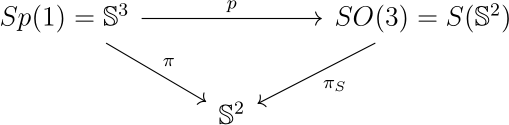
  is simply connected, it is not diffeomorphic to . However, the Hopf fibration can be regarded as the double cover of , in the sense that this diagram commutes
Here  is the double covering map from
  to . To see this, first identify with the compact symplectic group
  where
where  is the set of quaternions, where
  . We identify with the space of purely imaginary quaternions
  . Then we define
  by
by

It is clear that  . Under this identification, then
  as we identify
  with
with  . Let
. Let  , where
  . Suppose
  ,
,  . Then by a direct calculation (done by Mathematica here)

On the other hand, for ,  can be defined to be

Expanding the above, we have

Comparing with (1), we have proved the commutativity.

 is the unit circle centered at
  on the plane and
  is a concentric circle with radius
  (
( ), what is the probability that a random triangle inscribed in
  is replaced by a general line segment inside the unit circle.
  and
and  are said to be independent if
  for all Borel sets
  . We don’t have a probability measure behind the abstract definition of noncommutative probability space, so we cannot define independence in this way. However, it is not difficult to show that the above definition is equivalent to the following: for any Borel-measurable functions
  such that
  are integrable, one has
 ![\mathbf{E}[f(X)g(Y)] = \mathbf{E}[f(X)] \mathbf{E}[g(Y)]](https://s0.wp.com/latex.php?latex=%5Cmathbf%7BE%7D%5Bf%28X%29g%28Y%29%5D+%3D+%5Cmathbf%7BE%7D%5Bf%28X%29%5D+%5Cmathbf%7BE%7D%5Bg%28Y%29%5D+&bg=ffffff&fg=000000&s=0&c=20201002) . Since we have an expectation in noncommutative context (namely
. Since we have an expectation in noncommutative context (namely  in the
  be a noncommutative probability space. Let
  be two subalgebras such that
  . We say that
  and
and  are classically independent if
 if
if  ,
, and
and  with
with  , then
  .
. and
and  , one has
  (by applying the definition to
  ). So this is indeed the same as the independence we saw in classical probability.
 , one can define the space of (essentially) bounded random variables
  , and a linear functional
  on this space, namely the expected value. So we may study the algebra
  -algebras are more important.
 , where
  is a complex algebra with a unit, and
  is a linear map such that
  .
. . To see that this is not a meaningless generalization, we can look at the following examples.
 ,
,  is a noncommutative probability space.
 with
with  .
. with
with  .
. , fix a unit vector
  with
with  and define
  . Then
  always denotes the geodesic ball of radius
  its boundary, which is called the geodesic sphere. In geodesic polar coordinates, let the area element of
 is the Jacobian (with respect to polar coordinates). For our purpose it is more convenient to regard
  as a one-parameter family of functions in the variable
  satisfies the
  )
) 
 is the
  is the arc-length parametrized
  starting from
  along
along  is a
is a 
 is the arclength parameter)
 is the
  . (Indeed, the differential version
  is already true for the geodesic circle.) This implies

 ,
,  , find a line in
  represented by
  that fits the data in the following sense. The loss of each data point
  to the line is
 for every
  ,
, that minimizes the loss function
![\displaystyle \sum_{i=1}^N [y_i - (mx_i + c)]^2.](https://s0.wp.com/latex.php?latex=%5Cdisplaystyle+%5Csum_%7Bi%3D1%7D%5EN+%5By_i+-+%28mx_i+%2B+c%29%5D%5E2.&bg=ffffff&fg=333333&s=0&c=20201002)
 . Then the new least squares problem can be formulated as follows.
 where
where  . Thus the distance between
  for every
  that minimizes the loss function
 .
.
 be the
  -dimensional
 .
. and define the
  by
by

 (analogous to the fact that the
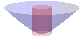
  , is a surface with constant curvature
  ). It is easy to see that
 ![\displaystyle \begin{array}{rl} \displaystyle X(\theta, \phi)= (r\sinh \theta \cos \phi,r \sinh \theta \sin \phi, r\cosh \theta), \quad \theta\ge 0, \quad \phi\in[0, 2\pi],\end{array}](https://s0.wp.com/latex.php?latex=%5Cdisplaystyle+%5Cbegin%7Barray%7D%7Brl%7D+%5Cdisplaystyle+X%28%5Ctheta%2C+%5Cphi%29%3D+%28r%5Csinh+%5Ctheta+%5Ccos+%5Cphi%2Cr+%5Csinh+%5Ctheta+%5Csin+%5Cphi%2C+r%5Ccosh+%5Ctheta%29%2C+%5Cquad+%5Ctheta%5Cge+0%2C+%5Cquad+%5Cphi%5Cin%5B0%2C+2%5Cpi%5D%2C%5Cend%7Barray%7D+&bg=ffffff&fg=000000&s=0&c=20201002)
 , with
  being the (geodesic) distance from
  .
.

 from
from  to
to 

 )
)
 is exactly the finite cylinder

 , the
, the 

 .
. )
)
 , i.e.
  is
is
 . He also showed that the volume of a ball of radius
  using the
  as shown.
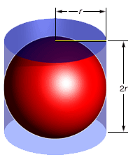
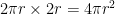
 plane, which then becomes a circle of radius
 is the “infinitesimal” increment of the angle
  sign),
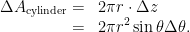

 ) is (see Fig.

 .
. , we have
  , which (up to a sign) is the rigorous version of
  , where the coefficients are random, what can we say about the distribution of the roots (on
  )? Of course, it would depend on what “random” means. Here, “random” means that the sequence
  is an i.i.d. sequence of complex random variables.
 , then as
  , the roots will tend to be distributed on the unit circle! (There are lots of interesting discussions
  , we have
 ,
, is the Lebesgue measure on the complex plane. We will also assume two basic potential theoretic results without proofs, namely
 , we write
  , the normalized counting measure. We define the expected normalized counting measure,
 ![\mathbf{E}[Z_{p_n}]](https://s0.wp.com/latex.php?latex=%5Cmathbf%7BE%7D%5BZ_%7Bp_n%7D%5D&bg=ffffff&fg=000000&s=0&c=20201002) , as follows. For any
, as follows. For any  ,
,![\displaystyle \begin{array}{rl} \displaystyle (\mathbf{E}[Z_{p_n}],\psi) &:= \mathbf{E}[(Z_{p_n}, \psi)]\\ &\displaystyle =\frac{1}{\pi^{n+1}}\int_{\mathbb{C}^{n+1}} \frac{1}{n}\sum_{j=1}^n \psi(\zeta_j)e^{-\sum_{j=0}^n |a_j|^2} \,\text{d}m(a_0)\cdots\text{d}m(a_n). \end{array}](https://s0.wp.com/latex.php?latex=%5Cdisplaystyle+%5Cbegin%7Barray%7D%7Brl%7D+%5Cdisplaystyle+%28%5Cmathbf%7BE%7D%5BZ_%7Bp_n%7D%5D%2C%5Cpsi%29+%26%3A%3D+%5Cmathbf%7BE%7D%5B%28Z_%7Bp_n%7D%2C+%5Cpsi%29%5D%5C%5C%C2%A0+%26%5Cdisplaystyle+%3D%5Cfrac%7B1%7D%7B%5Cpi%5E%7Bn%2B1%7D%7D%5Cint_%7B%5Cmathbb%7BC%7D%5E%7Bn%2B1%7D%7D+%5Cfrac%7B1%7D%7Bn%7D%5Csum_%7Bj%3D1%7D%5En+%5Cpsi%28%5Czeta_j%29e%5E%7B-%5Csum_%7Bj%3D0%7D%5En+%7Ca_j%7C%5E2%7D+%5C%2C%5Ctext%7Bd%7Dm%28a_0%29%5Ccdots%5Ctext%7Bd%7Dm%28a_n%29.+%5Cend%7Barray%7D+&bg=ffffff&fg=000000&s=0&c=20201002)
 are distributed “on average”.
![\displaystyle \lim_{n\to\infty} \mathbf{E}[Z_{p_n}] = \frac{1}{2\pi}\text{d}\theta](https://s0.wp.com/latex.php?latex=%5Cdisplaystyle+%5Clim_%7Bn%5Cto%5Cinfty%7D+%5Cmathbf%7BE%7D%5BZ_%7Bp_n%7D%5D+%3D+%5Cfrac%7B1%7D%7B2%5Cpi%7D%5Ctext%7Bd%7D%5Ctheta+&bg=ffffff&fg=000000&s=0&c=20201002)

 is a solution to
  (usually denoted by “
 ”, but indeed there is no single-valued square root for complex numbers, or even negative real numbers).
 and
and  :
: 
 in the first expansion and comparing with the remaining two, it’s easy to see that


 with the point
  on the plane. We can write a complex number in its polar form
  , which is identified with
  in polar coordinates. We call
  and
and  the
the  respectively.
 and
and  is then
 is the product of the two moduli and the argument of
  and compute
 . We will argue that its length is
  and its argument is

 . Then
  and so
![\displaystyle \begin{array}{rl} \displaystyle |({z_n})^n| =|z_n|^n =\left(1+\frac{x^2}{n^2}\right)^{\frac{n}{2}} =& \displaystyle \left[\left(1+\frac{x^2}{n^2}\right)^{n^2}\right]^{\frac{1}{2n}}\\ \rightarrow& \displaystyle \left(e^{x^2}\right)^{0}=1 \ \ \ \ \ (3)\end{array}](https://s0.wp.com/latex.php?latex=%5Cdisplaystyle+%5Cbegin%7Barray%7D%7Brl%7D+%5Cdisplaystyle+++%7C%28%7Bz_n%7D%29%5En%7C+%3D%7Cz_n%7C%5En+%3D%5Cleft%281%2B%5Cfrac%7Bx%5E2%7D%7Bn%5E2%7D%5Cright%29%5E%7B%5Cfrac%7Bn%7D%7B2%7D%7D+%3D%26+%5Cdisplaystyle+%5Cleft%5B%5Cleft%281%2B%5Cfrac%7Bx%5E2%7D%7Bn%5E2%7D%5Cright%29%5E%7Bn%5E2%7D%5Cright%5D%5E%7B%5Cfrac%7B1%7D%7B2n%7D%7D%5C%5C+%5Crightarrow%26+%5Cdisplaystyle+%5Cleft%28e%5E%7Bx%5E2%7D%5Cright%29%5E%7B0%7D%3D1++%5C+%5C+%5C+%5C+%5C+%283%29%5Cend%7Barray%7D+&bg=ffffff&fg=000000&s=0&c=20201002)
 . On the other hand, the argument of
  (which is well-defined up to a multiple of
  ) can be chosen to be

![\displaystyle \begin{array}{rl} \displaystyle \lim_{n\rightarrow \infty} \arg [(z_n)^n ]= \lim_{n\rightarrow \infty} n\arg(z_n)= \lim_{n\rightarrow \infty} n\theta_n=x. \ \ \ \ \ (4)\end{array}](https://s0.wp.com/latex.php?latex=%5Cdisplaystyle+%5Cbegin%7Barray%7D%7Brl%7D+%5Cdisplaystyle++%5Clim_%7Bn%5Crightarrow+%5Cinfty%7D+%5Carg+%5B%28z_n%29%5En+%5D%3D+%5Clim_%7Bn%5Crightarrow+%5Cinfty%7D+n%5Carg%28z_n%29%3D+%5Clim_%7Bn%5Crightarrow+%5Cinfty%7D+n%5Ctheta_n%3Dx.+%5C+%5C+%5C+%5C+%5C+%284%29%5Cend%7Barray%7D+&bg=ffffff&fg=000000&s=0&c=20201002)

 (but without giving the full mathematical details) in the above approach:
 function
  on
on  such that
 ![{[c_1,c_2]\subset f(\mathbb R^2)}](https://s0.wp.com/latex.php?latex=%7B%5Bc_1%2Cc_2%5D%5Csubset+f%28%5Cmathbb+R%5E2%29%7D&bg=ffffff&fg=000000&s=0&c=20201002) and
and ![{f^{-1}([c_1,c_2])}](https://s0.wp.com/latex.php?latex=%7Bf%5E%7B-1%7D%28%5Bc_1%2Cc_2%5D%29%7D&bg=ffffff&fg=000000&s=0&c=20201002) is compact, we have
is compact, we have 
 .
.
 is compactly supported, then
